Advanced Time Series Analysis: State Space Models and Kalman Filtering

Time series analysis is a powerful tool for understanding and predicting the behavior of data that evolves over time. State space models and Kalman filtering are advanced techniques that allow us to model and estimate the underlying states of a system based on noisy observations. In this tutorial, we will explore the concepts of state space models and Kalman filtering and implement them in Python.

Photo by Dmitry Mashkin on Unsplash

Table of Contents

1. Introduction to State Space Models
2. The Kalman Filter Algorithm
3. Implementing State Space Models and Kalman Filtering in Python
4. Case Study: Predicting Stock Prices using State Space Models and Kalman Filtering
5. Conclusion

1. Introduction to State Space Models

State space models provide a flexible framework for modeling time series data. They consist of two components: the state equation and the observation equation. The state equation describes how the underlying states of the system evolve over time, while the observation equation relates the observed data to the underlying states.

The state equation can be represented as follows:

x(t) = F(t) * x(t-1) + G(t) * u(t)

where x(t) is the state vector at time t, F(t) is the state transition matrix, x(t-1) is the state vector at time t-1, G(t) is the control matrix and u(t) is the control vector.

The observation equation can be represented as follows:

y(t) = H(t) * x(t) + v(t)

where y(t) is the observed data at time t, H(t) is the observation matrix, x(t) is the state vector at time t and v(t) is the observation noise.

State space models allow us to capture complex dynamics and dependencies in the data, making them suitable for a wide range of applications, including finance, economics and engineering.

2. The Kalman Filter Algorithm

The Kalman filter is an algorithm used to estimate the underlying states of a system based on noisy observations. It operates recursively, updating the state estimate as new observations become available.

The Kalman filter algorithm consists of two steps: the prediction step and the update step.

Prediction Step

In the prediction step, we use the state equation to predict the next state based on the current state estimate:

x_hat(t|t-1) = F(t) * x_hat(t-1|t-1) + G(t) * u(t)
P(t|t-1) = F(t) * P(t-1|t-1) * F(t)^T + Q(t)

where x_hat(t|t-1) is the predicted state estimate at time t, x_hat(t-1|t-1) is the previous state estimate at time t-1, P(t|t-1) is the predicted state covariance at time t, P(t-1|t-1) is the previous state covariance at time t-1 and Q(t) is the process noise covariance.

Update Step

In the update step, we use the observation equation to update the state estimate based on the new observation:

K(t) = P(t|t-1) * H(t)^T * (H(t) * P(t|t-1) * H(t)^T + R(t))^-1
x_hat(t|t) = x_hat(t|t-1) + K(t) * (y(t) - H(t) * x_hat(t|t-1))
P(t|t) = (I - K(t) * H(t)) * P(t|t-1)

where K(t) is the Kalman gain at time t, R(t) is the observation noise covariance, x_hat(t|t) is the updated state estimate at time t, y(t) is the new observation at time t and I is the identity matrix.

The Kalman filter provides an optimal estimate of the underlying states given the observations and the model assumptions. It is widely used in various fields, including signal processing, control systems and finance.

3. Implementing State Space Models and Kalman Filtering in Python

Now that we have a good understanding of state space models and the Kalman filter algorithm, let’s implement them in Python. We will use the numpy library for numerical computations and the matplotlib library for data visualization.

Installing Required Libraries

Before we begin, let’s install the required libraries. Open your terminal and run the following command:

pip install numpy matplotlib

Importing Required Libraries

Once the libraries are installed, we can import them in our Python script:

import numpy as np
import matplotlib.pyplot as plt

Generating Synthetic Data

To demonstrate the implementation of state space models and Kalman filtering, let’s generate some synthetic data. We will create a simple linear system with Gaussian noise.

np.random.seed(0)

# Define the number of time steps
T = 100

# Define the state transition matrix
F = np.array([[1]])

# Define the observation matrix
H = np.array([[1]])

# Define the process noise covariance
Q = np.array([[0.1]])

# Define the observation noise covariance
R = np.array([[1]])

# Define the initial state
x0 = np.array([0])

# Generate the true state and observations
x_true = np.zeros((T, 1))
y = np.zeros(T)

x_true[0] = x0
y[0] = H @ np.asarray(x_true[0]) + np.random.multivariate_normal(np.zeros((1,)), R)

for t in range(1, T):
    x_true[t] = F @ x_true[t-1] + np.random.multivariate_normal(np.zeros((1,)), Q)
    y[t] = H @ np.asarray(x_true[t]) + np.random.multivariate_normal(np.zeros((1,)), R)

Implementing the Kalman Filter

Now that we have the synthetic data, let’s implement the Kalman filter algorithm to estimate the underlying states.

# Initialize the state estimate and covariance
x_hat = np.zeros((T, 1))
P = np.zeros((T, 1, 1))

x_hat[0] = x0
P[0] = Q

# Run the Kalman filter
for t in range(1, T):
    # Prediction step
    x_hat[t] = F @ x_hat[t-1]
    P[t] = F @ P[t-1] @ F.T + Q

    # Update step
    K = P[t] @ H.T @ np.linalg.inv(H @ P[t] @ H.T + R)
    x_hat[t] = x_hat[t] + K @ (y[t] - H @ x_hat[t])
    P[t] = (np.eye(1) - K @ H) @ P[t]

Visualizing the Results

Finally, let’s visualize the true states, observations and estimated states using the Kalman filter.

# Plot the true states, observations and estimated states
plt.figure(figsize=(10, 6))
plt.plot(range(T), x_true, label='True States')
plt.plot(range(T), y, label='Observations')
plt.plot(range(T), x_hat, label='Estimated States')
plt.xlabel('Time')
plt.ylabel('State')
plt.legend()
plt.show()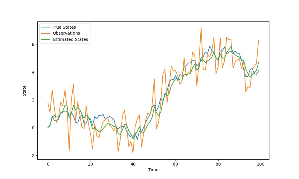

Figure 1: True States, Observations and Estimated States

In Figure 1, we can see that the estimated states closely track the true states, even in the presence of noise.

4. Case Study: Predicting Stock Prices using State Space Models and Kalman Filtering

Now that we have a basic understanding of state space models and Kalman filtering, let’s apply these techniques to a real-world problem: predicting stock prices.

Downloading Stock Price Data

To begin, we need to download stock price data for a specific asset. We will use the yfinance library to download the data. Run the following code to install the library:

pip install yfinance

Once the library is installed, we can download the stock price data using the following code:

import yfinance as yf

# Download stock price data
data = yf.download('JPM', start='2020-01-01', end='2023-11-30')

Preprocessing the Data

Before we can apply state space models and Kalman filtering, we need to preprocess the stock price data. We will convert the data into log returns, which are more suitable for modeling financial time series.

# Compute log returns
data['Log Returns'] = np.log(data['Close']).diff()

# Remove missing values
data = data.dropna()

Building the State Space Model

Next, we need to build the state space model for predicting stock prices. We will use a simple model with a constant drift and a random walk for the volatility.

# Define the state transition matrix
F = np.array([[1]])

# Define the observation matrix
H = np.array([[1]])

# Define the process noise covariance
Q = np.array([[0.001]])

# Define the observation noise covariance
R = np.array([[0.01]])

# Define the initial state
x0 = np.array([0])

# Define the number of time steps
T = len(data)

# Generate the observations
y = data['Log Returns'].values.reshape(-1, 1)

Estimating the States using the Kalman Filter

Now that we have the state space model and the observations, let’s estimate the underlying states using the Kalman filter.

# Initialize the state estimate and covariance
x_hat = np.zeros((T, 1))
P = np.zeros((T, 1, 1))

x_hat[0] = x0
P[0] = Q

# Run the Kalman filter
for t in range(1, T):
    # Prediction step
    x_hat[t] = F @ x_hat[t-1]
    P[t] = F @ P[t-1] @ F.T + Q

    # Update step
    K = P[t] @ H.T @ np.linalg.inv(H @ P[t] @ H.T + R)
    x_hat[t] = x_hat[t] + K @ (y[t] - H @ x_hat[t])
    P[t] = (np.eye(1) - K @ H) @ P[t]

Visualizing the Results

Finally, let’s visualize the true log returns, estimated log returns and predicted stock prices.

# Compute the estimated log returns
log_returns_hat = x_hat.flatten()

# Compute the predicted stock prices
prices_hat = np.exp(np.cumsum(log_returns_hat))

# Plot the true log returns, estimated log returns and predicted stock prices
plt.figure(figsize=(10, 6))
plt.plot(data.index, data['Log Returns'], label='True Log Returns')
plt.plot(data.index, log_returns_hat, label='Estimated Log Returns')
plt.plot(data.index, prices_hat, label='Predicted Prices')
plt.xlabel('Date')
plt.ylabel('Log Returns / Prices')
plt.legend()
plt.show()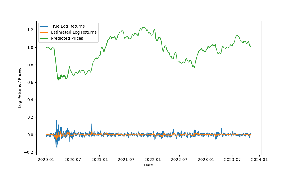

Figure 2: True Log Returns, Estimated Log Returns and Predicted Prices

In Figure 2, we can see that the estimated log returns closely track the true log returns and the predicted prices follow the general trend of the true prices.

5. Conclusion

In this tutorial, we explored the concepts of state space models and Kalman filtering for advanced time series analysis. We implemented state space models and the Kalman filter algorithm in Python and applied them to a case study of predicting stock prices.

State space models and Kalman filtering are powerful tools for modeling and estimating the underlying states of a system based on noisy observations. They have wide-ranging applications in various fields, including finance, economics and engineering.

By understanding and applying these techniques, you can gain valuable insights into the dynamics of time series data and make more accurate predictions. Experiment with different models and data to further enhance your understanding and explore the full potential of state space models and Kalman filtering.